How it works#
This page follows a chart through the package, from a formula to a picture. It explains what is computed at each step and why. The other pages show how to use each part; this one describes what happens inside, and links back to them for usage.
The process has five stages, and each one produces what the next one needs:
| stage | produces | source |
|---|---|---|
| construction | a chart whose every scale is a curve | construct.jl, compound.jl, net.jl, fan.jl |
| automatic construction | the same, from a formula | auto.jl, auto_chain.jl |
| solving | values, and the lines that read them | solve.jl |
| layout | a NomogramDrawing: pure geometry |
ticks.jl, drawing.jl |
| rendering | SVG, or a Makie Figure |
svg.jl, ext/NomogramsMakieExt.jl |
All of these stages use the same representation of a chart, so that comes first.
One condition: collinearity#
A nomogram rests on a single condition: a point taken from each scale lies on one straight line exactly when the values satisfy the relation. For three points this is d'Ocagne's criterion (see the Bibliography),
and nothing else about the picture affects what it computes. So the package stores each scale as a parametric curve, value -> (x, y), over a domain. A Scale holds a Variable (name, label, tick preferences), the domain it covers, that curve, the side its ticks go on, and a kind: :scale for a scale that a reader takes values from, or :grid for a strand of a Net. A Nomogram is a list of scales, a canvas size, a title, and optionally the algebraic relation that the scales are meant to encode.
The curves do not have to come from a construction. Three scales built by hand, with v twice as far from u as w is and w at half scale, chart u + v = w. A line between heights 10u and 10v crosses the middle at their average, 5(u + v).
using Nomograms

u = Scale(Variable(:u; domain = (0, 10)), (0.0, 10.0), u -> (0.0, 10u), :left)
v = Scale(Variable(:v; domain = (0, 10)), (0.0, 10.0), v -> (70.0, 10v), :right)
w = Scale(Variable(:w; domain = (0, 20)), (0.0, 20.0), w -> (35.0, 5w), :right)
sum3 = Nomogram([u, v, w]; width = 70, height = 100)
drawing(sum3; isopleths = [isopleth(sum3; u = 3, v = 4, label = "3 + 4")])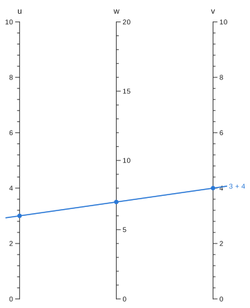
align_residual computes the determinant. It is the cross product of q − p with point − p, which is twice the signed area of the triangle formed by the three points. It is zero on the line and grows linearly away from it:
p, q = point(u, 3), point(v, 4)
(align_residual(w, 7, p, q), align_residual(w, 8, p, q))
(0.0, 350.0)Because every chart comes down to a set of scales, everything after construction (solving, ticks, labels and both renderers) is written once, in terms of the curves. Nomogram, CompoundNomogram and NetNomogram differ only in how they are solved. For drawing, all three are an AbstractNomogram: scales, a canvas and a title.
Construction: choosing the curves#
Each constructor chooses curves in a particular way that makes the determinant agree with a relation. Building charts shows them in use; this section describes what each one computes.
Parallel scales. additive_nomogram charts f₁(u) + f₂(v) = f₃(w) in closed form. The outer scales go on x = 0 and x = W at heights a₁(f₁ − p₀) and a₂(f₂ − q₀), with each gradient chosen to fit its transform's range to the canvas height. A line between them crosses x = λW at (1 − λ)y₁ + λy₂, and choosing λ = a₁ / (a₁ + a₂) makes that a linear function of f₁ + f₂. So the middle axis's position and gradient are determined by the outer two. Its domain is determined the same way: the reachable range of f₃ is [p₀ + q₀, p₁ + q₁], mapped back through the result's inverse transform. If a domain was given, it is checked against that range instead.
The middle axis lies close to whichever outer axis spans more. When the gradients differ by more than max_modulus_ratio (4 by default), the steeper one is capped by shortening that axis and centring it. Shifting an outer axis by d shifts every crossing of the middle one by d times that axis's share of the width, so the middle axis is shifted to match and no reading changes. multiplicative_nomogram wraps every transform in a logarithm and calls additive_nomogram.
The N-chart. ratio_nomogram puts f₁ up the left edge and f₂ down the right, and reads the ratio on the diagonal between their zero corners. A line through the two crosses the diagonal at s = kr / (kr + 1), where r = f₁/f₂ and k is the ratio of the two gradients. This is a projective scale, which is why a ratio spanning several decades gets decade-based ticks on the diagonal.
Curves you supply. determinant_nomogram takes one curve per variable, in whatever coordinates are convenient. It samples each curve at 129 points to measure the combined bounding box, and maps that box onto the canvas with an affine map, using separate factors for the two axes unless preserve_aspect is set. An affine map keeps collinear points collinear, so the fit cannot change an answer. Each scale's ticks go on the side whose normal points away from the centre of the canvas, so labels face outwards on a curve as they do on a parallel chart.
Reshaping. project composes every curve with a homography and fits the result to the canvas with the same affine step. projective_transform finds the homography from four point pairs by solving the 8 × 8 linear system their coordinates give. If the map sends a point to infinity, the error names the scale that point lies on. fan is a projective map chosen to bring the meeting point of parallel axes onto the page, so the axes become spokes. It builds both orientations, with each axis's top at the rim and at the hub, and keeps the one that labels more ticks.
Chains. compound places each later stage with a similarity (rotation, uniform scaling and translation) that carries its copy of the shared scale onto the copy already placed. The similarity is computed as one complex division, from the shared scale's points at a quarter and three quarters of its domain. It is then checked at 17 points along the whole domain, because the two copies are not guaranteed to have the same shape. Finally the stages are translated together to the origin and their scales are listed from left to right.
Nets. A Net is a surface (u, v) -> (x, y) that fills one of the three points on the alignment line. It is drawn as strands: for each round value of one variable, the curve traced by the other. Each strand is an ordinary Scale of kind :grid, so the drawing code needs nothing extra. Four or more variables derives the condition a net has to meet.
Every construction that knows its relation stores it in the chart. This is what allows max_relation_residual to solve the chart over a grid of inputs and compare each answer with the relation.
Solving: where a line crosses a curve#
Reading a chart, whether by eye or with evaluate, answers one question: where does the line through the known points cross the unknown's scale?
The solver first checks that exactly one variable is missing and that every known value is inside its scale's domain. It then takes the points on two known scales as p and q. The unknown is a root of v -> align_residual(scale, v, p, q) on that scale's domain. solve_all_on finds every root using Roots.find_zeros, instead of bracketing one root between the ends of the domain. A straight scale gives a residual that is linear in position, and so at most one root. A curved scale can give several, and each one is a valid solution. The search runs slightly past each end of the domain, where the curve is still defined, and then clamps back, so that a root lying exactly on an end is not lost to rounding.
evaluate then requires a single answer, and throws an error listing them if there are more. evaluate_all returns them all, and isopleth returns the single line with every crossing marked. Solving shows each of these.
The other chart types reduce to this case. A CompoundNomogram is solved by propagation: any stage with exactly one unknown is read, its answer is added to the known values, and the pass repeats until nothing is left or no stage can be solved. So any set of inputs that closes the chain works, from either end. A NetNomogram with both net variables known contributes one fixed point, and the problem is the ordinary one. If one of them is unknown, the two scales fix the line, and the answer is where the line crosses the strand of the known net variable. That strand is a curve, so it may be crossed twice.
From a formula#
auto_nomogram builds all of the above from a function. From a formula gives the mathematics; this section gives the order in which things happen.
Wrapping the formula. The function is first put behind a FunctionWrapper with a fixed signature, (Float64, …) -> Float64, one for each number of inputs. Every Julia closure has its own type, so code specialised on it would be compiled again for each formula. With the wrapper, the code is compiled once, and precompile.jl runs the common paths when the package is precompiled, so that compiled code is already cached. The original function is kept as well, for the one step that has to differentiate it automatically.
Testing separability. For two inputs, separability_defect evaluates L = ln|F_x / F_y| on a 9 × 9 grid inset 2% from the edges of the domain. It then measures the worst violation of the rectangle identity
about the middle of the grid. The derivatives are central differences whose step scales with the argument as well as the domain. At the edges they switch to one-sided formulas, so F is never called outside the domain it was given. If the defect is above 1e-6, the formula has no chart on three straight scales, and the search for a curved scale (described below) takes over. The same happens if a derivative changes sign, since a straight scale cannot fold back.
Recovering the transforms. If the identity holds, F_x / F_y = f′(x) / g′(y). Holding y at the middle of its domain gives f′, and holding x there gives g′, each up to the same constant. Each is integrated with five-point Gauss–Legendre quadrature over 256 panels. The panels are spaced geometrically when the domain spans more than a decade, since that is where a log-like integrand changes fastest. The result is stored as a TabulatedScale: values and exact derivatives at the nodes, joined by cubic Hermite interpolation and extended linearly past the ends.
growth = auto_nomogram((r, n) -> (1 + r / 100)^n, :rate => (1, 20), :years => (1, 30), :growth)
growth[:rate].variable.transform
TabulatedScale(257 nodes on [1, 20])The result's transform h would need F to be inverted. To avoid that, the package walks a straight path across the domain from the corner where F is smallest to the corner where it is largest. Along that path both inputs move in the direction that increases F, so F increases steadily. The path parameter is solved for at 1025 values of F, and at each one h = f + g, with h′ from the chain rule. The three transforms are fixed only up to a common sign, which is chosen so that the result axis reads upwards. Each axis's tick style is also chosen at this point, according to how its transform spreads its values.
Checking. The transforms are passed to additive_nomogram, with F itself stored as the chart's relation. The finished chart is then solved on a 9 × 9 grid of inputs, and every answer is compared with F. If any answer differs by more than rtol times the result's range, the chart is not returned.
One curved scale. When straight scales fail, each variable is tried on a curve in turn, starting with the result. Write the relation as G(u, v, w) = 0 with w on the curve. Near each level w = c, w(u, v) is found by Newton's method in whatever number type it is given. This means ForwardDiff dual numbers pass straight through and come out with exact derivatives of the implicit function. On 25 level sets, with 11 points each, L_uv is fitted as A w_u w_v + B w_uv. A relative misfit above 1e-6 on any of them rules out that arrangement. The fitted B(c) is tabulated, and the log-slopes a′ = L_u − B w_u and b′ = −(L_v − B w_v) are integrated twice with the same quadrature as above. Then 161 levels, spaced more closely toward the ends of the range, each give one line g = m f + k from one point on their level set. With f on the axis x = 0 and g on x = 1, every alignment line for that level passes through (1/(1 − m), k/(1 − m)), and these points are tabulated as the curve. The three scales are passed to determinant_nomogram and checked on the same 9 × 9 grid.
Chains. With three or more inputs, each pair (xᵢ, xⱼ) is tested as a possible first stage: does F depend on that pair only through one combination of them? That holds exactly when F_i / F_j does not change with the other inputs. The test evaluates the log of that ratio on a 5 × 5 grid of the pair, and compares it across three settings of each of the other inputs. If the pair passes, the combination T is F with the other inputs held at their midpoints, charted by the two-input method onto an unmarked turning line. The remainder G(t, rest…) needs, for each t, some point where T = t. The same rising path is tabulated once against t, so each call of G costs an interpolation instead of a root search. G is then charted the same way, recursively, until two inputs are left.
The stages are joined with compound. It fails, and the pairing is rejected, when two stages need the turning line on scales of different shapes, as (a + b)·c does. The layout is searched at the same time. For the first two levels of the chain, every workable pairing is built, and the one whose narrowest gap between neighbouring axes is widest, relative to the chart's width, is kept. Deeper levels take the first pairing that works, since the number of options multiplies with every level. Each earlier stage has one input that lands inside the rest of the chain. That stage is mirrored and resized, to between a quarter of the final stage's width and all of it, to put that input midway between the axes already there. The assembled chain is checked as a whole against F on a grid of four values per input.
Layout: from curves to geometry#
drawing turns a chart into a NomogramDrawing: polylines, tick marks with their normals and label anchors, titles, and isopleth segments. Everything is in chart units, with y pointing up. The steps run in a fixed order, because each step reserves space that later steps must respect.
Paths. Each scale is sampled at 129 points. If every sample lies on the chord, the path is reduced to its two end points, as happens for every axis of a parallel chart.
Titles. Axis titles are placed before any ticks, clear of each other and of the axis lines of every other scale a reader uses. Each title first tries a position off the end of its axis, continuing the direction of the curve. It tries the higher end first, then the other, then steps further out from both. A position far enough out is always clear, so the search always ends, and it ends in a position that overlaps nothing. A title is never drawn on top of another or across an axis.
Ticks. For each scale,
candidate_ticksoffers values that are round in the variable, in order of importance: decades before 5s before 2s on a log axis, multiples of 10 before multiples of 5 on a linear one, and the user's order for explicitticks.thin_ticksthen places them in that order. The ends of the domain go first if they are numbers someone chose (at most three significant figures). Any value that would land too close on the page to one already placed is rejected. As a result, a compressed stretch of a reciprocal or log axis keeps fewer labels, and the ones it keeps are the roundest. Drawing covers the tick rules in more detail.Isopleth segments. Each alignment line runs from its leftmost to its rightmost crossing, extended by
isopleth_overhangat each end. Only the part between the crossings is checked against labels.Collisions across the chart. Thinning compares a scale only with itself, so one more pass is made over the whole chart. It takes major labels, then minor ones, and keeps each label only if its box overlaps nothing already reserved, no alignment line crosses it, and it does not sit across another scale's axis.
segment_hits_boxdoes the line tests by clipping. A rejected label is removed and its tick mark is kept. Text boxes are estimated from the label's length, size, alignment and rotation (label_box), without font metrics, so the layout is the same whichever backend draws it.Isopleth labels. You asked for these explicitly, so they are moved instead of dropped.
nudge_cleartries the end of the line, then steps to either side of it along the perpendicular until the label is clear.Chart title and bounds. The bounding box is enlarged to cover everything placed, and the chart title is centred above it.
The result is plain data, which you can inspect directly:
d = drawing(sum3)
[(sd.name, length(sd.ticks), count(t -> !isnothing(t.label), sd.ticks)) for sd in d.scales]
3-element Vector{Tuple{Symbol, Int64, Int64}}:
(:u, 26, 6)
(:v, 26, 6)
(:w, 21, 5)d.scales[3].ticks[end]Nomograms.TickMark(20.0, (35.0, 100.0), (1.0, -0.0), 1.5, "20", 1, (37.3, 100.0), (:left, :center), 0.0)Each TickMark holds its value, position, outward normal, length, label and level, plus the anchor, alignment and rotation of its text. That is everything a renderer needs to put the text where the layout placed it.
Rendering#
Both backends walk over a NomogramDrawing, and neither makes any layout decisions of its own. svg writes the SVG document directly, with no dependencies. It converts chart units to pixels using pxperunit, flips y, draws the paths, ticks and isopleths, and places each label from its anchor and alignment. Isopleths take their colour from a three-colour palette, and from the fourth on their dash pattern changes as well, so a reading is never identified by colour alone. Drawing explains this choice. The Makie backend, nomogramplot, is in a package extension that loads when a Makie backend is loaded, and draws the same structure into an Axis.

Charts and drawings also define show for image/svg+xml. This is how a notebook, VS Code, or a page like this one displays them automatically.